

how to find probability with mean and standard deviation
vi.3: Finding Probabilities for the Normal Distribution
- Page ID
- 5194
The Empirical Dominion is just an approximation and only works for certain values. What if you want to find the probability for ten values that are not integer multiples of the standard deviation? The probability is the area under the curve. To detect areas under the curve, you need calculus. Before engineering science, you lot needed to catechumen every x value to a standardized number, called the z-score or z-value or simply just z. The z-score is a mensurate of how many standard deviations an x value is from the hateful. To convert from a unremarkably distributed x value to a z-score, you utilize the following formula.
Definition \(\PageIndex{1}\): z-score
\[z=\dfrac{x-\mu}{\sigma} \label{z-score}\]
where \(\mu\)= hateful of the population of the x value and \(\sigma\)= standard departure for the population of the 10 value
The z-score is normally distributed, with a mean of 0 and a standard divergence of ane. It is known as the standard normal curve. Once y'all accept the z-score, you can wait upwards the z-score in the standard normal distribution table.
Definition \(\PageIndex{two}\): standard normal distribution
The standard normal distribution, z, has a hateful of \(\mu =0\) and a standard deviation of \(\sigma =ane\).
.png?revision=1)
Luckily, these days technology can find probabilities for you without converting to the zscore and looking the probabilities upwards in a table. In that location are many programs available that will calculate the probability for a normal curve including Excel and the TI-83/84. At that place are also online sites available. The following examples evidence how to do the calculation on the TI-83/84 and with R. The control on the TI-83/84 is in the DISTR menu and is normalcdf(. You lot then blazon in the lower limit, upper limit, mean, standard deviation in that guild and including the commas. The command on R to observe the area to the left is pnorm(z-value or x-value, mean, standard deviation).
Example \(\PageIndex{1}\) full general normal distribution
The length of a human pregnancy is normally distributed with a mean of 272 days with a standard departure of nine days (Bhat & Kushtagi, 2006).
- State the random variable.
- Find the probability of a pregnancy lasting more than 280 days.
- Find the probability of a pregnancy lasting less than 250 days.
- Find the probability that a pregnancy lasts between 265 and 280 days.
- Detect the length of pregnancy that 10% of all pregnancies last less than.
- Suppose you encounter a woman who says that she was meaning for less than 250 days. Would this exist unusual and what might you lot retrieve?
Solution
a. x = length of a man pregnancy
b. Commencement translate the statement into a mathematical statement.
P (10>280)
At present, draw a picture. Retrieve the center of this normal bend is 272.
.png?revision=1)
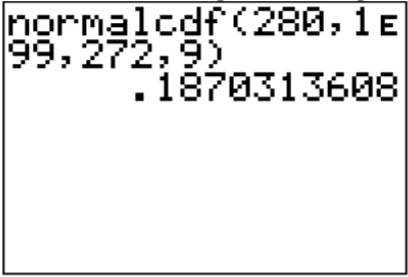
To find the probability on the TI-83/84, looking at the movie you realize the lower limit is 280. The upper limit is infinity. The reckoner doesn't have infinity on it, then you lot need to put in a really large number. Some people like to put in one thousand, only if you are working with numbers that are bigger than one thousand, then yous would have to remember to change the upper limit. The safest number to use is \(1 \times ten^{99}\), which you put in the figurer equally 1E99 (where E is the EE button on the calculator). The command looks similar:
\(\text{normalcdf}(280,1 E 99,272,9)\)
.png?revision=1)
To find the probability on R, R always gives the probability to the left of the value. The full area nether the curve is 1, so if you want the expanse to the right, and then you find the surface area to the left and subtract from 1. The command looks like:
\(i-\text { pnom }(280,272,9)\)
Thus, \(P(x>280) \approx 0.187\)
Thus eighteen.seven% of all pregnancies terminal more than 280 days. This is not unusual since the probability is greater than 5%.
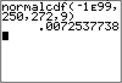
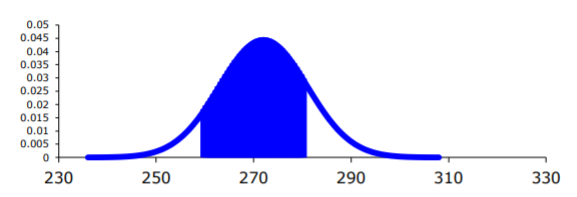
c. Showtime translate the statement into a mathematical argument.
P (x<250)
Now, draw a picture. Remember the eye of this normal curve is 272.
.png?revision=1)
To observe the probability on the TI-83/84, looking at the picture, though information technology is hard to see in this case, the lower limit is negative infinity. Again, the reckoner doesn't have this on information technology, put in a actually modest number, such as \(-1 \times 10^{99}=-1 E 99\) on the calculator.
.png?revision=1)
\(P(x<250)=\text { normalcdf }(-i E 99,250,272,9)=0.0073\)
To find the probability on R, R ever gives the probability to the left of the value. Looking at the figure, you can see the surface area you want is to the left. The control looks like:
\(P(x<250)=\text { pnorm }(250,272,ix)=0.0073\)
Thus 0.73% of all pregnancies last less than 250 days. This is unusual since the probability is less than v%.
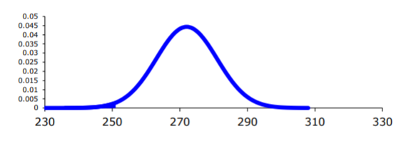
d. First translate the statement into a mathematical statement.
P (265<x<280)
Now, depict a motion picture. Retrieve the centre of this normal curve is 272.
.png?revision=1)
In this case, the lower limit is 265 and the upper limit is 280.
Using the figurer
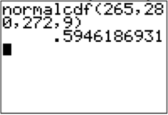.png?revision=1)
\(P(265<10<280)=\text { normalcdf }(265,280,272,9)=0.595\)
To use R, yous have to remember that R gives you the surface area to the left. Then \(P(x<280)=\text { pnom }(280,272,9)\) is the area to the left of 280 and \(P(x<265)=\text { pnom }(265,272,9)\) is the area to the left of 265. So the area is between the two would be the bigger i minus the smaller one. So, \(P(265<x<280)=\text { pnorm }(280,272,9)-\text { pnorm }(265,272,ix)=0.595\). Thus 59.5% of all pregnancies last between 265 and 280 days.
e. This problem is asking you to find an x value from a probability. Y'all desire to find the 10 value that has 10% of the length of pregnancies to the left of it. On the TI-83/84, the command is in the DISTR menu and is called invNorm(. The invNorm( command needs the area to the left. In this instance, that is the area you are given. For the command on the estimator, once y'all take invNorm( on the master screen y'all type in the probability to the left, mean, standard difference, in that order with the commas.
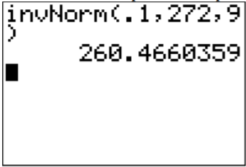.png?revision=1)
On R, the command is qnorm(surface area to the left, hateful, standard deviation). For this example that would be qnorm(0.i, 272, 9)
Thus 10% of all pregnancies concluding less than approximately 260 days.
f. From part (c) you found the probability that a pregnancy lasts less than 250 days is 0.73%. Since this is less than 5%, it is very unusual. You would recall that either the adult female had a premature baby, or that she may exist wrong almost when she really became pregnant.
Case \(\PageIndex{2}\) full general normal distribution
The mean mathematics SAT score in 2012 was 514 with a standard divergence of 117 ("Total group profile," 2012). Assume the mathematics SAT score is ordinarily distributed.
- Land the random variable.
- Find the probability that a person has a mathematics SAT score over 700.
- Find the probability that a person has a mathematics SAT score of less than 400.
- Find the probability that a person has a mathematics Saturday score between a 500 and a 650.
- Find the mathematics SAT score that represents the summit 1% of all scores.
Solution
a. x = mathematics SAT score
b. Commencement translate the statement into a mathematical argument.
P (x>700)
Now, draw a picture. Remember the center of this normal curve is 514.
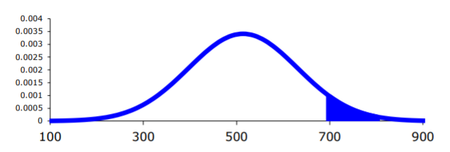.png?revision=1)
On TI-83/84: \(P(x>700)=\text { normalcdf }(700,1 Eastward 99,514,117) \approx 0.056\)
On R: \(P(ten>700)=1-\text { pnorm }(700,514,117) \approx 0.056\)
At that place is a five.6% gamble that a person scored higher up a 700 on the mathematics SAT test. This is not unusual.
c. Showtime translate the statement into a mathematical statement.
P (x<400)
Now, describe a picture. Call back the center of this normal bend is 514.
.png?revision=1)
On TI-83/84: \(P(ten<400)=\text { normalcdf }(-1 E 99,400,514,117) \approx 0.165\)
On R: \(P(ten<400)=\operatorname{pnorm}(400,514,117) \approx 0.165\)
And so, there is a sixteen.5% hazard that a person scores less than a 400 on the mathematics part of the Sabbatum.
d. Start interpret the statement into a mathematical statement.
P (500<x<650)
Now, depict a moving-picture show. Remember the heart of this normal bend is 514.
.png?revision=1)
On TI-83/84: \(P(500<x<650)=\text { normalcdf }(500,650,514,117) \approx 0.425\)
On R: \(P(500<x<650)=\text { pnorm }(650,514,117)-\text { pnorm }(500,514,117) \approx 0.425\)
So, in that location is a 42.5% gamble that a person has a mathematical Saturday score betwixt 500 and 650.
due east. This problem is request yous to find an x value from a probability. You lot want to find the x value that has 1% of the mathematics Sat scores to the right of it. Recollect, the calculator and R always need the expanse to the left, you need to find the area to the left by 1 - 0.01 = 0.99.
On TI-83/84: \(\text{invNorm}(.99,514,117) \approx 786\)
On R: \(\text{qnorm}(.99,514,117) \approx 786\)
Then, 1% of all people who took the Sabbatum scored over about 786 points on the mathematics SAT.
Homework
Practise \(\PageIndex{1}\)
- Find each of the probabilities, where z is a z-score from the standard normal distribution with mean of \(\mu =0\) and standard departure \(\sigma =1\). Make sure you draw a picture for each problem.
- P (z<ii.36)
- P (z>0.67)
- P (0<z<2.11)
- P (-2.78<z<1.97)
- Notice the z-score corresponding to the given area. Call up, z is distributed equally the standard normal distribution with mean of \(\mu =0\) and standard deviation \(\sigma =1\).
- The surface area to the left of z is xv%.
- The area to the right of z is 65%.
- The area to the left of z is ten%.
- The area to the correct of z is 5%.
- The area betwixt -z and z is 95%. (Hint draw a motion-picture show and figure out the area to the left of the -z.)
- The surface area between -z and z is 99%.
- If a random variable that is normally distributed has a mean of 25 and a standard deviation of 3, convert the given value to a z-score.
- 10 = 23
- x = 33
- x = 19
- 10 = 45
- According to the WHO MONICA Project the mean blood pressure for people in Red china is 128 mmHg with a standard deviation of 23 mmHg (Kuulasmaa, Hense & Tolonen, 1998). Assume that blood pressure is normally distributed.
- Land the random variable.
- Find the probability that a person in People's republic of china has blood pressure of 135 mmHg or more.
- Notice the probability that a person in China has blood pressure of 141 mmHg or less.
- Find the probability that a person in China has blood pressure betwixt 120 and 125 mmHg.
- Is information technology unusual for a person in China to have a blood pressure of 135 mmHg? Why or why not?
- What claret pressure practice 90% of all people in China have less than?
- The size of fish is very important to commercial angling. A study conducted in 2012 found the length of Atlantic cod caught in nets in Karlskrona to have a mean of 49.9 cm and a standard deviation of 3.74 cm (Ovegard, Berndt & Lunneryd, 2012). Assume the length of fish is commonly distributed.
- Country the random variable.
- Find the probability that an Atlantic cod has a length less than 52 cm.
- Find the probability that an Atlantic cod has a length of more than 74 cm.
- Observe the probability that an Atlantic cod has a length between xl.five and 57.5 cm.
- If you found an Atlantic cod to have a length of more 74 cm, what could you conclude?
- What length are 15% of all Atlantic cod longer than?
- The mean cholesterol levels of women age 45-59 in Ghana, Nigeria, and Seychelles is 5.i mmol/l and the standard departure is 1.0 mmol/l (Lawes, Hoorn, Police force & Rodgers, 2004). Assume that cholesterol levels are normally distributed.
- Country the random variable.
- Find the probability that a woman age 45-59 in Ghana, Nigeria, or Seychelles has a cholesterol level above 6.two mmol/l (considered a loftier level).
- Find the probability that a woman age 45-59 in Republic of ghana, Nigeria, or Republic of seychelles has a cholesterol level below 5.2 mmol/l (considered a normal level).
- Find the probability that a woman historic period 45-59 in Ghana, Nigeria, or Seychelles has a cholesterol level betwixt v.2 and 6.two mmol/l (considered borderline high).
- If you found a woman historic period 45-59 in Republic of ghana, Nigeria, or Republic of seychelles having a cholesterol level higher up half-dozen.2 mmol/fifty, what could you conclude?
- What value practice v% of all woman ages 45-59 in Republic of ghana, Nigeria, or Seychelles have a cholesterol level less than?
- In the Usa, males betwixt the ages of forty and 49 eat on average 103.1 g of fat every day with a standard deviation of iv.32 k ("What we swallow," 2012). Assume that the amount of fatty a person eats is ordinarily distributed.
- State the random variable.
- Find the probability that a man historic period 40-49 in the U.Due south. eats more than than 110 one thousand of fat every 24-hour interval.
- Discover the probability that a man age twoscore-49 in the U.S. eats less than 93 g of fat every twenty-four hour period.
- Find the probability that a man age forty-49 in the U.South. eats less than 65 g of fat every day.
- If you establish a man age 40-49 in the U.S. who says he eats less than 65 m of fat every day, would you believe him? Why or why not?
- What daily fat level practise 5% of all men historic period 40-49 in the U.S. eat more than?
- A dishwasher has a mean life of 12 years with an estimated standard difference of i.25 years ("Appliance life expectancy," 2013). Assume the life of a dishwasher is usually distributed.
- Land the random variable.
- Find the probability that a dishwasher volition last more than than xv years.
- Notice the probability that a dishwasher will concluding less than vi years.
- Detect the probability that a dishwasher will last between 8 and 10 years.
- If you institute a dishwasher that lasted less than 6 years, would you call back that you have a trouble with the manufacturing procedure? Why or why not?
- A manufacturer of dishwashers but wants to supercede free of charge 5% of all dishwashers. How long should the manufacturer make the warranty period?
- The mean starting bacon for nurses is $67,694 nationally ("Staff nurse -," 2013). The standard difference is approximately $x,333. Assume that the starting bacon is normally distributed.
- State the random variable.
- Find the probability that a starting nurse will brand more than $80,000.
- Detect the probability that a starting nurse will make less than $60,000.
- Find the probability that a starting nurse will make between $55,000 and $72,000.
- If a nurse made less than $50,000, would yous think the nurse was under paid? Why or why not?
- What bacon exercise 30% of all nurses make more than?
- The hateful yearly rainfall in Sydney, Australia, is about 137 mm and the standard deviation is well-nigh 69 mm ("Annual maximums of," 2013). Presume rainfall is normally distributed.
- State the random variable.
- Discover the probability that the yearly rainfall is less than 100 mm.
- Find the probability that the yearly rainfall is more than 240 mm.
- Find the probability that the yearly rainfall is between 140 and 250 mm.
- If a year has a rainfall less than 100mm, does that mean it is an unusually dry year? Why or why not?
- What rainfall amount are xc% of all yearly rainfalls more than?
- Respond
-
1. a. \(P(z<2.36)=0.9909\), b. \(P(z>0.67)=0.2514\), c. \(P(0<z<two.11)=0.4826\), d. \(P(-2.78<z<1.97)=0.9729\)
3. a. -0.6667, b. -two.6667, c. -two, d. six.6667
5. a. See solutions, b. \(P(ten<52 \mathrm{cm})=0.7128\), c. \(P(ten>74 \mathrm{cm})=five.852 \times 10^{-xi}\), d. \(P(twoscore.5 \mathrm{cm}<x<57.five \mathrm{cm})=0.9729\), e. See solutions, f. 53.8 cm
7. a. See solutions, b. \(P(x>110 \mathrm{g})=0.0551\) c. \(P(10<93 \mathrm{g})=0.0097\), d. \(P(10<65 \mathrm{1000}) \approx 0\) or \(v.57 \times 10^{-xix}\), east. Come across solutions, f. 110.2 yard
nine. a. See solutions, b. \(P(10>\$ 80,000)=0.1168\), c. \(P(ten>\$ 80,000)=0.2283\), d. \(P(\$ 55,000<x<\$ 72,000)=0.5519\), e. Run across solutions, f. $73,112
Source: https://stats.libretexts.org/Bookshelves/Introductory_Statistics/Book:_Statistics_Using_Technology_%28Kozak%29/06:_Continuous_Probability_Distributions/6.03:_Finding_Probabilities_for_the_Normal_Distribution
Posted by: davisexter1987.blogspot.com
0 Response to "how to find probability with mean and standard deviation"
Post a Comment